


 Français
Understanding > Knowing more > Asteroids and comets I
PANORAMA
ON ASTEROIDS
Introduction
The discovery of asteroids
In January 1801, while he was building a stellar catalog, the Italian astronomer Giuserppe Piazzi discovered a moving object over the fixed stars background. He first thought he had discovered a new comet. Once the orbit of this new object had been determined circular and confined between Mars and Jupiter, it became however obvious that it was not a comet. Indeed, all comets have highly eccentric orbits.
Piazzi therefore thought he had discovered the "missing planet" predicted by the pseudo-numerical Titius-Bode law. In 1766, Johannes Titius realized that the semi-major axis of planets' orbit followed a geometric sequence. A few years later, Johann Elert Bode popularized this sequence: distance (au) = 0.4 + 0.3 x 2n, with n=-∞, 0, 1, 2... for the different planets (Mercury, Venus, the Earth, Mars... see Table 1).
This numerological law, without physical basis, found some notoriety after the discovery of Uranus by William Herschel in 1781. This new planet, the first since Antiquity, was indeed located on an orbit very close to the n=6 prediction (see Table 1). The Titius-Bode pseudo-law was also predicting a planet (n=3) at 2.8 au from the Sun. Many astronomers were then convinced that an unknown planet was located between Mars and Jupiter. Piazzi thus concluded that the new object he had discovered was a planet, which he dumbed Cerere Fernandinae, in the name of the Sicilian god of agriculture, and the king Ferdinand of Sicily. The name of Fernandinae was quickly abandonned, and the new planet known under the name of Ceres.
While the astronomer Heinrich Olbers was trying to observe Ceres to characterize its orbit, he discovered another body in March 1802. This object, dumbed Pallas by Olbers, was located on an orbit very close to that of Ceres. This second discovery suggested that the single and large planet predicted by the Titius-Bode law had been destructed. Several small plaets could thus exist in its place. The discovery of Juno (1804) and Vesta (1809), and of tens of others objects in the following years, conforted this idea. William Herschel proposed since 1802 the name of asteroids ("like a star") to design these objects.
What are asteroids?
For long, asteroids remained terra incognita. Being point-like sources moving over the stellar background, the asteroids were called the "vermins of the sky" during the first half of the twentieth century. Astronomers indeed considered as a disturbance the small streaks they imprinted on photographic plates.
Nowadays, we know that asteoroids are rocky bodies no larger than a few hundreds of kilometers (Ceres, by far the largest, has a diameter of 950 km). The smallest have diameters of only a few centimeters (for smaller fragments, we generally speak of "dust").
Astronomers in the early ninetieth century thought asteroids were the remnants of a planet destruction. We now understood that asteroids are the building blocks of planets, and they are the witnesses of the early stages of our solar system (cf I).
Asteroids display a wide diversity. They are located everywhere in the solar system (cf II), with highly different shapes and sizes (cf III), and a wide range of compositions (cf IV).
I. Why do we study asteroids?
I.1. Witnesses of the primordial solar system
Owing to their small size, asteroids are geologically dead bodies. Although they experienced many collisions, their composition has remained constant since their formation, 4.5 Gyrs, within the disk of gas and dust within which the planets formed.
The planets are so big that the energy provided by the desintegration of radioactive nucleii is enough to melt rocks. The planets therefore differentiated, i.e., the most dense compounds sinked and formed a core. This energy, provided as heat, is responsible for the plate tectonic, and volcanism. All these mechanisms have masked the original composition of the Earth. In some case, the erosion by the atmosphere (Venus), or by the biosphere (Earth) add a second level of complexity. This is why the study of planets only cannot tell us about the material from which they formed.
On the other hand, the vast majority of asteroid are too small to have any internal enargy. They are therefore primitive bodies, with little evolution over the history of the solar system. Nowadays, they are the most-similar material to the bricks upon which planets formed. Studying asteroid composition hence directly informs us on the original compounds of telluric planets.
Moreover, the distribution of the different compositions of asteroid provides a glimpse of the first stages of our solar system. Indeed, from the study of exoplanets (planets orbiting other stars than the Sun) revealed that planets may form at a different location than their current orbit. The process of "migratio", during which the orbits of planets shrink due to their interaction with the surrounding disk, seems wellspread. The distributions of asteroid orbits, sizes, and compositions still contain information on these migrations.
I.2. Parent body of meteorites
Often, asteroids fall on Earth. The fragments that hit the ground are called meteorites. Their study has a double interest: understanding planet formation, and Earth protection.
The study of meteorites in the laboratory allows us to understand their composition, the conditions in which they formed, at which timescale did they accrete, etc. They are direct sample from asteroids. By connecting the different types of meteorites to the classes of asteroids, we understand better our History (cf II.1).
Nevertheless, these falls present a risk, especially for large asteroids. Only a few impact craters are visible on Earth, but it is due to the erosion (plate tectonic, water...), that erased them, rather than a lack of impacts. The miriad of craters on the Moon are here to remind us the threat represented by asteroid collisions. It is an asteroid, impacting the Earth on the Yucatan peninsula some 65 millions years ago, creating a 180 km wide crater, which is responsible for the mass extinction that killed dinosaurs.
More recently, a surface area of 2000 km2 in Siberia was devastated by the atmospheric explosion of a bolide of a few tens of meters. In 2013, over Chelyabinsk in Russia, the explosion of a small asteroid (about 20m diameter) produced numerous injuries to inhabitants, and serious material damages. About 1500 people were injuried, mostly by glass fragments verre (Figure 1).
I.3. The new Eldorado?
The comercial exploitation of asteroid is more and more seriously considered. Several private companies currently envision sending robotic space probes to explore, and then exploit near-Earth asteroids (cf II.1). Most asteroids are not richer in metal and rare elements (ore, nickel, lithium) than the Earth crust. Given the cost of developing, building, and sending a space probe, the buisness plan may not seem appealing.
Some asteroids are nevertheless enriched in heavy elements. During the first stages of planetary formation (see above, I.1), bodies accreted within the proto-planetary disk. Many planetary embryos, with diameters similar to Ceres at about 1000 km, were then formed. The existence of nickel-iron meteorites tells us that some of these bodies differentiated: dense material like metals formed a nucleus at the center, and lighter elements like rocks stayed above and formed a mantle and a crust. These proto-planets were then destroyed by impacts, and their fragments are spread in the asteroid main belt. The fragments from the nucleus could therefore contain billions of tons of metals (nickel, iron, cobalt, etc) per cubic kilometer! Such quantities are large enough to cover the world needs for centuries.
On a (ver much) longer time scale, asteroids could be advtantageous space bases to colonize the solar system. Indeed, their small sizes imply small masses, and taking off from an asteroid thus requires much less energy than from a planet. This is how asteroid resources could be used by settlers, including water, carbon, and nitrogen.
II. Where the asteroids are located?
II.1. Different populations
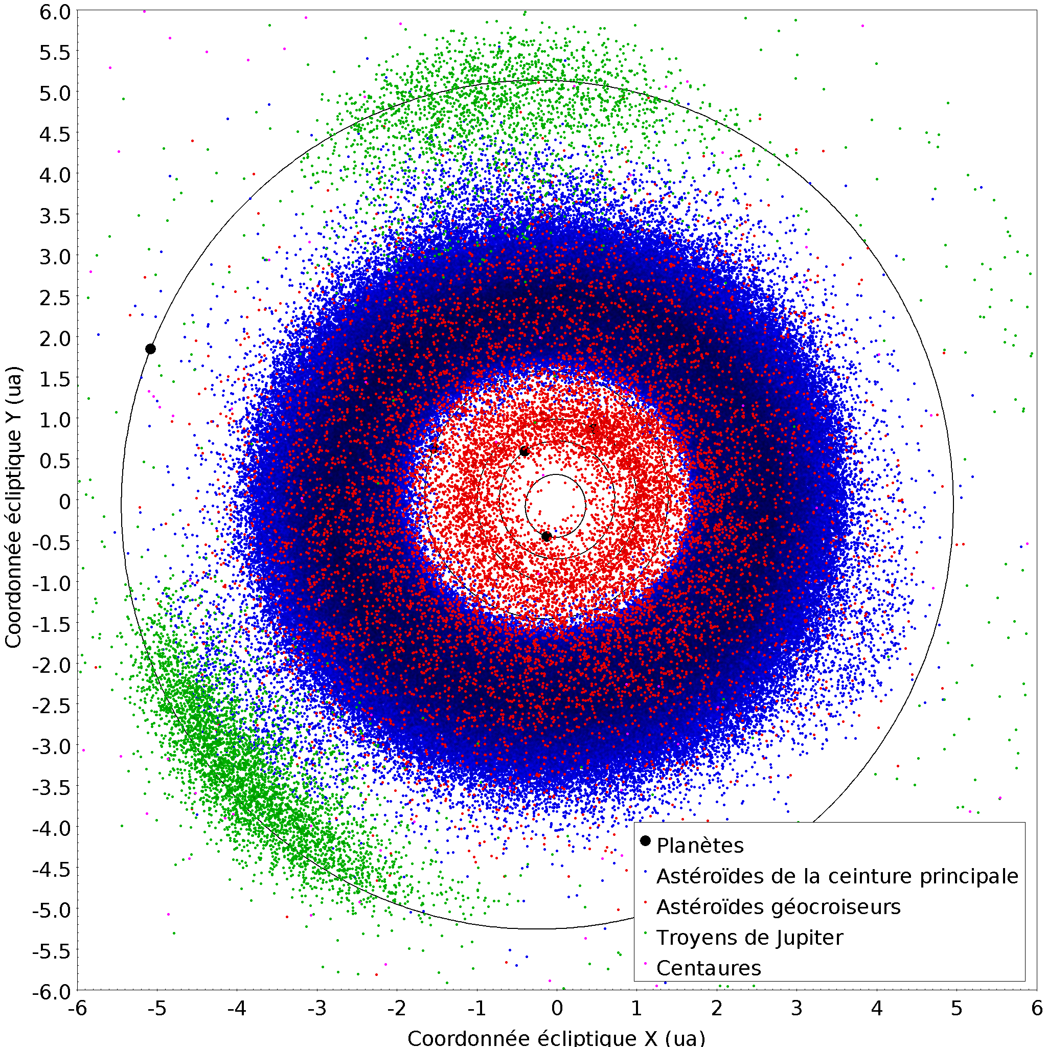
The first asteroid to be discovered, Ceres, orbits the Sun between Mars and Jupiter, at 2.8 au. Until 1898 and the discovery of (433) Eros which orbit crosses that of the Earth, all the asteroids were discovered in this region, now called the asteroid main belt. Asteroids with orbit alike Eros are called near-Earth asteroids. (Figure 2).
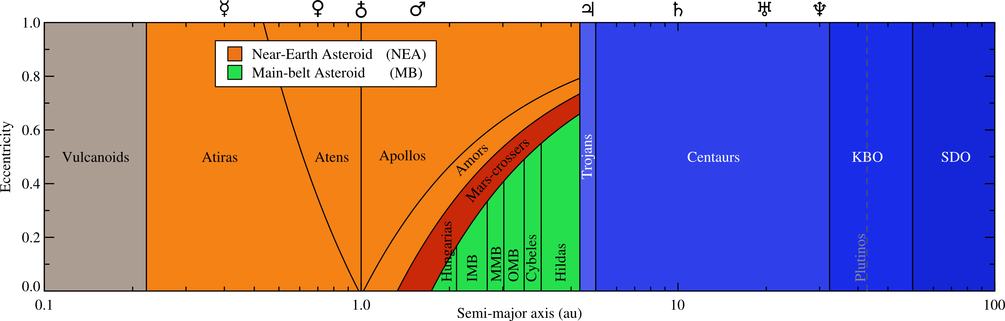
The main belt is the main reservoir of asteroids, with more than 700,000 known asteroids (July 2016), and likely more than a million with a diameter larger than 1 km. It is a stable region, where asteroids have been preserved over 4.5 Gyrs. We now believe giant planets have migrated over their history, and the asteroid main belt contains small bodies from the entire primordial solar system.
The near-Earth asteroids (NEAs) have a very short lifetime, of a few million years only, after which they are either ejected from the solar system, or they impact a planet or the Sun. These represent a direct threat for the Earth (cf I.2). This population is constantly replenished from the main belt, which sends new asteroids by several mechanisms (cf II.2). There are several sub-groups of NEAs, generally named after the first asteroid discovered in the group (defined by orbital properties): Atens, Apollos, Amors, Atiras, and Mars-Crossers (Table 2).
On Jupiter's orbit are the Trojans. These bodies follow or preceed Jupiter on its orbit with an angle of 60°, at the stable dynamical Lagrange points (defined with the three body problem). Jupiter's trojans are the largest population of trojans know, but all planets from the Earth to Neptune, have trojan asteroids.
Centaurs are the bodies which orbits cross that of the four giant planets. Alike the NEAs in the inner solar system, Centaurs have limited lifetime. This population is also constantly replenished, from the Edgeworth-Kuiper belt, beyond Neptune. Centaurs are the parent bodies of short-period comets (period of less than 200 years).
The Edgeworth-Kuiper belt is the second largest reservoir of small bodies, from 30 to 100 au. These cold objects are seldom called asteroids, and the names of transneptunian, or Kuiper-belt object (KBO) are favored. The existence of such a belt, made by a large number of small bodies, had been predicted by Edgeworth in 1949 and Kuiper in 1951, even if only one body was known there: Pluto (considered as a planet at that time, like Ceres at the time of its discovery). The discovery of the first KBO as such was made in 1992, quickly followed by many others. This motivated the change of status of Pluto from planet to dwarf-planet by the international astronomical union in 2006. Just like the asteroids of the main belt, Kuiper belt objects are the remnants of the early solar system.
Last, at the outskirts of the solar system is the Oort cloud, between 30,000 and 100,000 au. We never observed objects a such distances from the Sun, but such a reservoir is likely to exist: the long-period comets must come from somewhere!
II.2. Orbits and dynamics
The figure 3 shows the distribution of asteroids as function of the semi-major axis of their orbit. Several empty regions are visible on this figure. These gaps were first noticed by D. Kirkwood in 1867 and are due to the gravitational interaction with Jupiter. These gaps do not correspond to empty space (as visible in figure 4 where the entire space within the main belt is filled with asteroids), but rather to precise orbital periods. The dynamical effect responsible for these gaps is called resonance.

A resonance occurs whenever the orbital period of an asteroid is commensurable with that of Jupiter, that is: the orbital period of the asteroid is a factor p/(p+q) of Jupiter's orbital period, where p and q are integers. These mean-motion resonances are written (p+q):p. For instance, the 5:2 resonance implies asteroids which orbit five times the Sun for each two of Jupiter. Within a resonance, the same Sun-asteroid-Jupiter configuration occurs at each p turns of Jupiter (2 in the 5:2 resonance, 1 in the 3:1, etc). The asteroid thus repeatedly feels the gravity pull of Jupiter in a given direction, which tend to increase the excentricity of its orbit.
With higher excentricity, the probability to impact another asteroid or a planet raises. Asteroids within a resonance have therefore a limited lifetime of a few million years. This is why Kirkwood gaps are visible in the orbital distribution of main belt asteroids (but not in the belt: there are no regions totally devoid of asteroids).
Far from being simply an interesting academic subject, the resonances are the main source of near-Earth asteroids (cf II.1) and of meteorites. This mechanism is very effective, and there is no primordial bodies in the resonances. Parent bodies of NEAs and meteorites were recently "pushed" into the resonances by collisions or by the Yarkovsky effect (which increases or decreases the semi-major axis of an asteroid orbit due to the delayed emission of the heat from the Sun, see III.1 below).
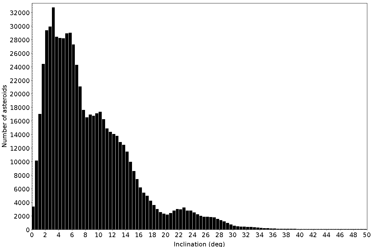
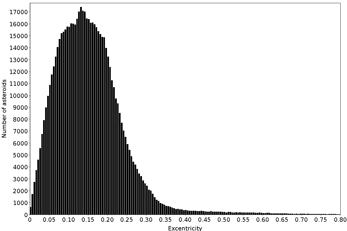
The distribution of inclination and eccentricity of asteroids are presented in figure 5. Overall, the orbits are all slightly inclined and excentric. This implies that collisions between asteroids are violent: typical collision occurs at 5 km/s in the main belt. This is what precludes the formation of a planet in this region.
II.3. Asteroids families
The study of asteroid orbital elements revealed another dynamical feature: groups of asteroids with very similar orbits. The first studies of these groups of asteroids, called families were initiated by Hirayama (1918) in the early twentieth century. These families are the result of collisions within the main belt.
Impacts of small asteroids on the largest only form craters, but the collision of two asteroids of similar size can lead to the entire destruction of one body or both. All the fragments will then share similar orbits around the Sun. There are currently 80 known families, from the proheminent and old (a few billion years old) Koronis or Eos families to the small and young (a few tens of thousands of years) Karin or Lucas-Cavin families Figure 6).
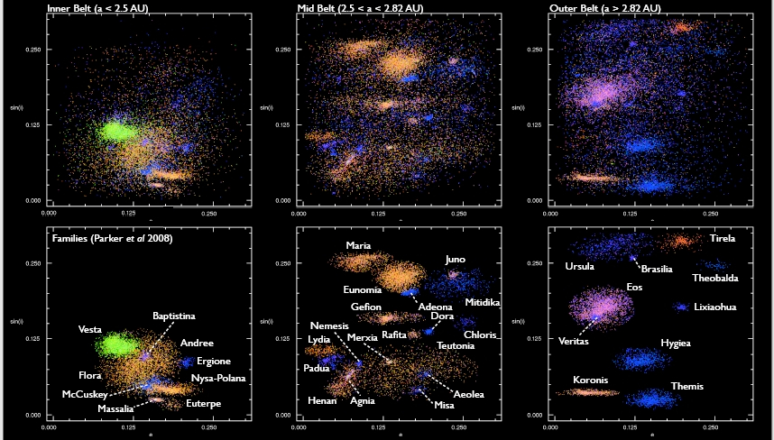
These families are extremely useful to understand surface properties of asteroids. Indeed, all the members of a family have the same age, being all the result of the cataclysmic collision that destroyed the parent body. Asteroid families allow us to study the "aging" of surfaces. It is the comparison of the surface properties of several families of similar composition but different ages that revealed the alteration of asteroid surfaces by the solar wind (seeIV.2).
III. What do asteroid look like?
III.1. Means of study
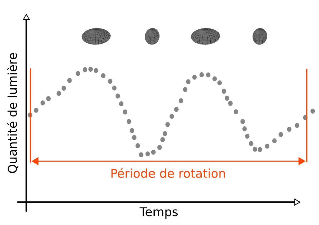
Lightcurves: The main way to study the rotation period and orientation of asteroids is the acquisition of lightcurves: the variation of the asteroid brightness as function of time. Because asteroids only reflect the sunlight (they do not produce light by themselves at visible wavelength) the quantity of light we measure (called photometry) is function of the apparent surface area of the asteroids. Over its rotation, this projected surface on the plane of the sky changes, and draws a sinusoidal curve (Figure 7). The rotation period can be directly measured on that curve and can be thus achieved in a night of observation. The rotation period is known for about 15,000 asteroids as of today (July 2016).
Determining the orientation of the spin axis requires more observations. To each Sun-asteroid-observer configuration corresponds a different lightcurve. It is easy to see that if the Earth is aligned with the spin axis the lightcurve will present no variation. On the contrary, its variation will be maximized if the Earth lays within the equatorial plane of the asteroid. Lightcurves taken in different geometry will have reduced amplitude, and different shapes. It is therefore requiered to collect lightcurves of the same body, under different Sun-asteroid-observer configurations, to determine the orientation of the spin axis. This is why this knowledge is still limited to a few hundreds of asteroids.
The shapes of the lightcurves being dictated by the apparent surface area of the asteroid over time, they can be used to reconstruct the 3-D shape of the asteroid (Kaasalainen et al. 2002, Durech et al. 2015). A single lightcurve is of course not enough. Many lightcurves, acquired under many different geometries must be collected. It is a complex problem that can lead to ambiguous solution. Yet, since early 2000s, it is the main source of 3-D shape models of asteroids. There are current a thousand asteroids with a shape model (see the DAMIT database, Durech et al. 2010).
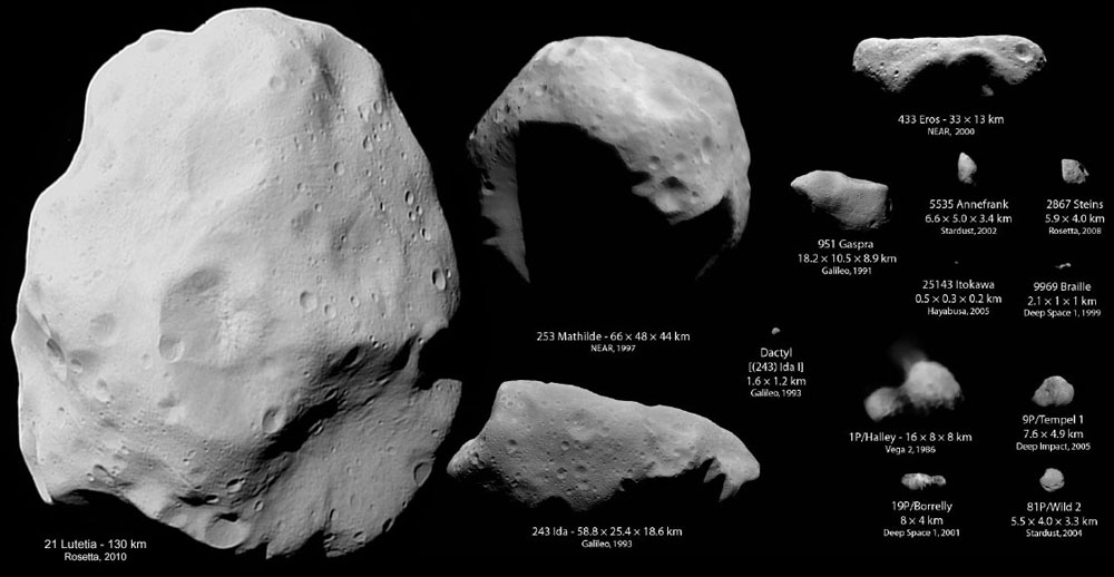
Direct imaging: Small bodies of the solar system are... small! Even the largest asteroid, (1) Ceres, has an angular diameter below the arcsecond (1°/3600). This is the angular size of a 2 Euros coin placed at 4 km. It is thus extremely difficult to directly image asteroids. Until the 1990s and the first flyby of an asteroid by a spaceprobe (Ida by Galileo on its way to Jupiter) asteroids had remained point-like sources.
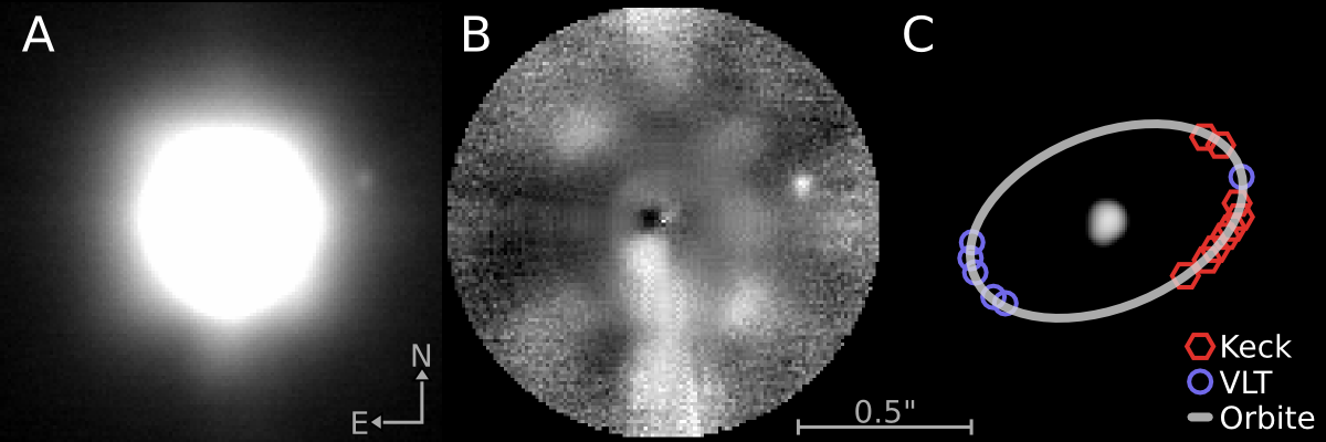
The main issue is the atmospheric turbulence, which "blurs" the images, degrading their resolution. The measure of this degradation is called the seeing. Even in favored sites, like the Mauna Kea on Hawai`i or the Atacama desert in Chile where the world's largest telescopes have been built, the seeing remains generally above one arcsecond. It is therefore impossible to observe small details. Thanksfully, a real-time correction has been invented in the late 1980s, called adaptive optics. With this technique, the first images of (1) Ceres and (2) Pallas were obtained in 1991 with the ESO 3.6m telescope (Saint-Pé et al. 1993). These were followed by many others once 10m class telescopes were operational: ESO VLT, Keck, Gemini. The Hubble space telescope, non affected by atmospheric turbulence thanks to its location above the atmosphere was also successfully used to image the two largest asteroids, (1) Ceres and (4) Vesta (Thomas et al. 1997).
The main interest of direct imaging is its repeatability. The second is the fact that it represents a direct measurement. Lightcurves allow to reconstruct the 3-D shape of an asteroid but only by stock-piling data for years. A few images taken over a night can provide the same result, each image providing the size and shape on the plane of the sky. Such images have been obtained on several tens of asteroids.
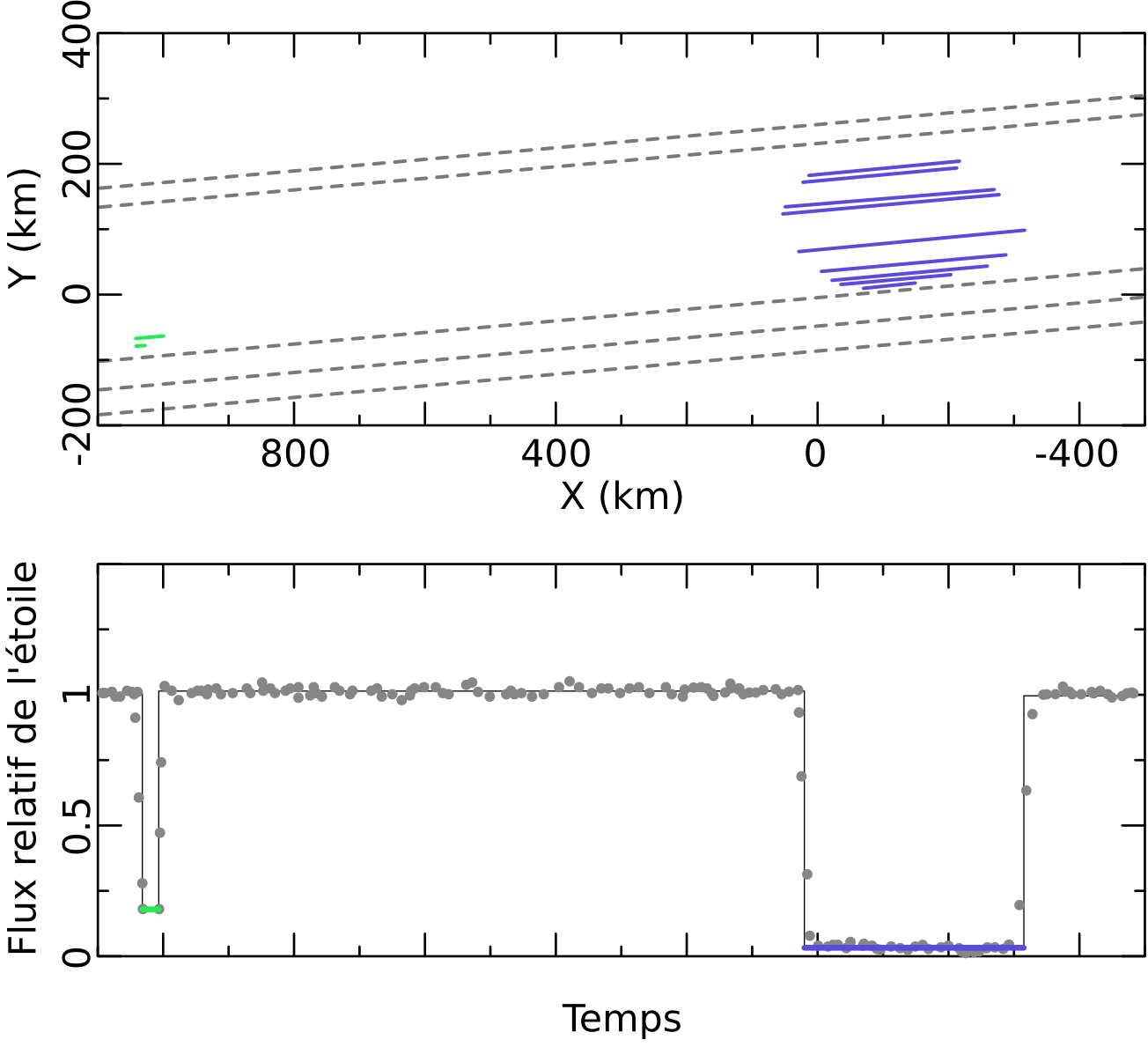
Stellar occultations: Another direct way to directly measure the apparent size and shape of asteroids consists in recording the duration of the disapparition of a star when an asteroid occults it. This duration can be converted into a length on the apparent disk of the asteroid, called a chord, by knowing its apparent speed, which is a direct by-product of our knowledge on its orbit. If several observers are located on the occultation path, several chords are measured and draw the apparent shape at the time of the stellar occultation.
This technique relies on a timing measurement, and can therefore be much more precise than direct imaging. Moreover, the observability of the occultations depends more on the star characeteristcs (mainly its apparent brightness) than of the occulting asteroid. Many targets too small angularly to be imaged (intrinsically small or very distant) can thus be studied by stellar occultations. However, because a given asteroid will only seldom occult a bright star, stellar occultations must be used in combination with other types of observations. Indeed, only a few asteroids have multiple recorded occultations with several chords, although more than 2000 stellar occultations were observed (mainly by amateur astronomers). Stellar occultations are a very good complement to lightcurves and can be used to reconstrct 3-D shapes (Carry et al. 2010, Kaasalainen 2011).
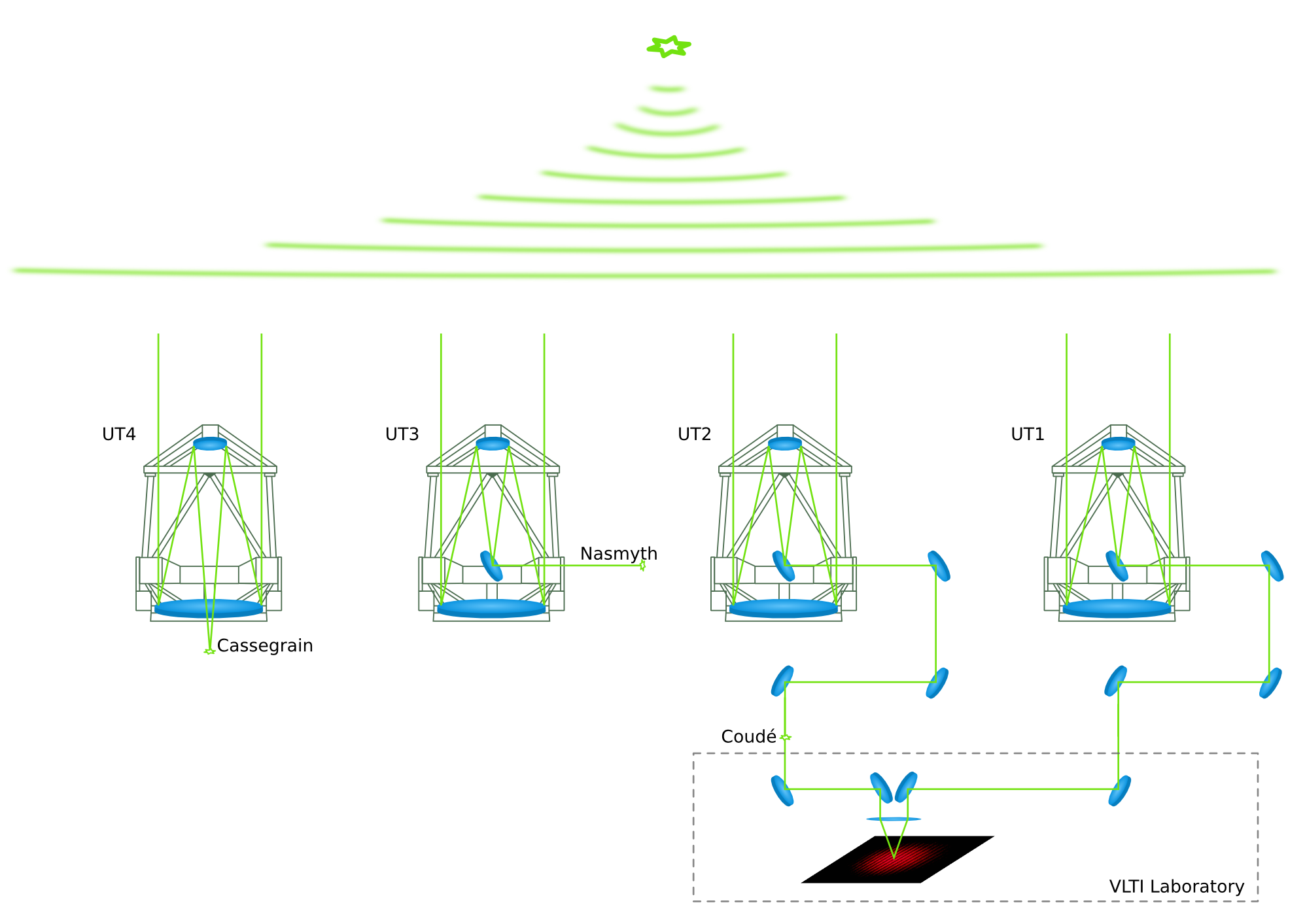
Interferometry: the angular resolution of images is limited by the atmospheric turbulence as discussed above. These effect can be corrected if the telescope or the camera are equipped with an adaptive-optics system. However, even in this case, the angular resolution will be limited by the diffraction, inverse proportional to the mirror size with the formula R = l/d, where l is the wavelength in meters, D the diameter of the primary mirror in meters, and R is the angular resolution in radians. As an example, the Hubble space telescope has the same angular resolution as the VLT telescopes, of about 0.05 arcsecond.
It is thus necessary to increase the mirror size D to improve the resolution. This becomes quickly expense and technically diffcult. A workaround consists in using two telescopes simultaneously, separated by a baseline B, and to combine the light they receive. Interference fringes appears, like in the Young experiment. The smallest detail observable is then l/B. The potential improvement is straightfoward: the VLT telescopes being separated by several tens of meters, their joint use provides an angular resolution ten times better than used separetedly.
This resolution is achieved along the line between the two telescopes only. There is no spatial information in other directions: interferometers do not take images. Moreover, this technique is limited to very bright objects: the combination of the two light beams is also disturbed by atmospheric turbulence, and only short integration times can be used. To date, only a few asteroids were studied using interferometry (Delbo et al. 2009, Carry et al. 2015). The technical aspect of interferometry are lower at longer wavelengths, and this technique seems highly promising for obsevratories like ALMA, collecting millimetric and sub-millimetric wavelength.
Radar echoes: Traditionnally, the measure of the position of asteroids to determine their orbit is done on images of stellar fields. The position is this a position on the plane of the sky, without information on the distance. By recording the time between the emission and reception of a radar signal echoed by an asteroid it is possible to measure its distance, and its velocity thanks to the Doppler-Fizeau effect .
Going further, by splitting the signal into delay and Doppler shift, provides informations on the rotation, size, and 3-D shape of the astroide. This information is not direct, but can reach a resolution of a few tens of meters only. Such a resolution by direct imaging requieres to be extremely close to the objects, as it occurs during spaceprobe flyby. Unfortunately, the energy of a radar echo being inverse proportional to the distance at the forth power, only objects coming very close to Earth ca be studied with radar echoes. Hence, only NEAs are studied with radar, when they close closer than 0.01 ua from Earth.
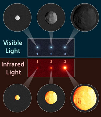
Radiometry in the thermal infrared: At visible wavelengths, the vast majority of the light we receive from asteroids comes from the reflection of the sunlight. In the infrared, the situation is different. Asteroid surfaces have typically temperatures of 200-300 K, and their blackbody radiation peaks around 10 microns. Measuring the flux at these wavelengths, and knowing the surface temperature, provides an estimate of the apparent diameter of the target.
This technique is the largest provider of asteroid diameters. The first catalogue of 2000 asteroid diameters was built in the 1980s using IRAS spaceprobe. The recent NASA WISE mission harvested a large amount of high-precision thermal fluxes, allowing the determination of the diameter of more than 150,000 asteroids from the NEAs to Jupiter Trojans. (ex. Masiero et al. 2011).
One of the limits of this technique comes from the modeling of the surface temperature. Many models exist, from simplistic models in which asteroids are represented by non-rotating sphere (e.g., the Standard Thermal Model, Lebofski et al. 1989), to complex models in which the 3-D shape, the rotation state, the granular aspect of the surface are taken into account (these are called thermophysical models). Depending on which model is used, the resulting diameter can be different. Results are thus unfortunately potentially biased, up to 10-20% in some pathological cases. The value of such catalogues is thus somehow limited for individual objects, also they are gold for statistical purposes.
III.2. Rotation period and orientation
The distribution of the rotation period and of the spin axis orientation of asteroids is not uniform, not isotrop. These two parameters bring many information, from the internal structure of asteroids, to non-ravitational forces, to the gas-pebble interactions within the proto-planetary nebula/
Spin-axis orientation: Among asteroids larger than 60 km in diameter, there is an exces of prograde rotator (spinning in the same sense as their motion around the Sun). This exces has been linked to the interaction between the disk of dust and gas in which they accreted (Johansen & Lacerda, 2010).
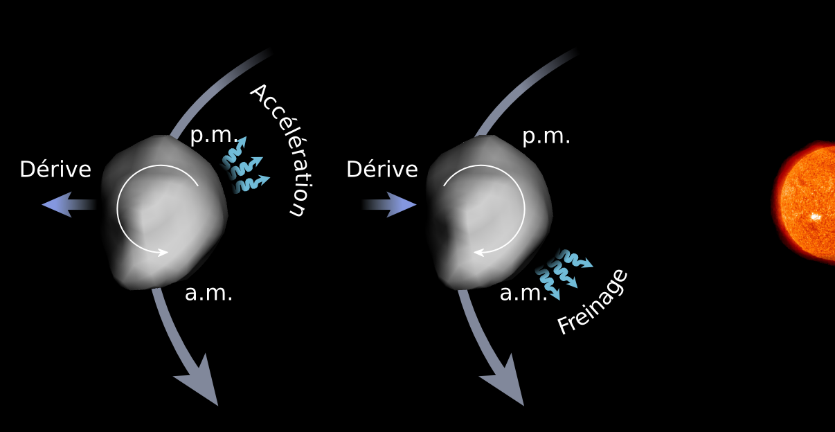
In asteroids smaller than 20 km in diameter, there is a concentration of the spin-axis orientation perpendicularly to their orbital plane. This is the result of the YORP effect (Yarkovsky-O'Keefe-Radzievskii-Paddack, see Figure 13). This effect is similar to the Yarkovsky effect described above in its mechanism (see II.2): the delayed thermal emission by the asteroid of the heat provided by the sunlight will preferentially orient asteroids in a "spinning top" configuration, either prograde or retrograde, but always with an obliquity close to 0° (Hanus et al., 2011, 2013).
Rotation period: The vast majority of asteroids spin in 4 to 10h. There are however some extremely slow rotators (rotation period of several days) and also extremely fast rotators (rotation period of a few minutes only!). The YORP effect described above is most likely responsible for these extreme periods. Another feature is the spin barrer, at about 2h that only monolithic asteroid can cross and spin faster. This barrer corresponds at a rotation state at which the surface particules are ejected: the rotation speed matches the liberation speed. Hence, only very small and solid asteroids, in which no matter can be ejected, are observed with shorter periods (Scheeres et al. 2015).
III.3. Size
The largest known asteroid, (1) Ceres, has a diameter of 935 km. By extending the term "asteroid" to all the small bodies of the solar system (the different names of the different population is mainly historical: they are all remnants of the planetary formation), the largest, (136108) Eris and (134340) Pluton, have diameters of about 2400 km. At the other end, the smallest bodies considered as asteroids have diameters of a few centimeters or tens of centimeters. Smaller bodies are generally refered to as dust. Such small bodies have never been observed directly, but the meteor showers are a direct evidence of their existance.
The size distribution of asteroids tells us about the dynamical processes that reign over their evolution. The size distribution of each population is well described by a power law. In the asteroid belt, this power law corresponds that of a theoretical power law for a population in collisional cascade (Dohnanyi 1969). Said differently, the collisions are the main processus which sculpt the main belt. The power law for Jupiter trojans and irregular satellites of giant planets are very different, and highlight a different history: these were captured during planetary migration (Morbidelli et al. 2005).
III.4. 3-D shape
Far from being spherical, asteroids present a large variety of shapes. The largest, like (1) Ceres and (4) Vesta, have reached hydrostatic equilibrium and their shape is close to an oblate sphere, like the Eeath. The shape of asteroids is however generally dictacted by the collisions they suffered over eons. Large craters have been imaged on every asteroid visited by spacecraft, sometimes with diameters as large as the asteroid!
The overall shape and internal structure is hence revelatory of the past of each asteroid. For instance, two impact bassins have been detected at the South pole of (4) Vesta, first with the Hubble space telescope (Thomas et al. 1997), then by the NASA Dawn mission (Russell et al. 2012). The most recent impact is the source of the asteroid family linked with Vesta, the Vestoids.
For the smallest asteroids, formed through collisions, the shape is highly irregular. These objects are likely the reaccumulation of a large number of fragments, hold together by gravity. These objects are called "rubble pile", such as the NEA (25143) Itokawa, visited by the Japanese mission Hayabusa.
III.5. Masse
The mass is the most difficult parameter to measure for an asteroid. These bodies are so small that their gravitational influence on other bodies is tiny compared to that of planets. The largest asteroids nevertheless perturb the orbit of Mars satellite, and small asteroids can be deflected during close encounters with more massive asteroids.
To measure the mass of an asteroid, its gravitational influence on another body must be detected, Close encounters between asteroids occur often and allowed to estimate the mass of 300 asteroids (see, e.g., Fienga et al. 2011). The accuracy of such determinations is however limited to date, owing to the complexity of the dynamical system to model, and of the limited quality of the astrometric positions of asteroids.
A much more accurate mass can be determined from the orbital study of a satellite, either natural or articifial (Figure 14). This is how the mass of asteroid visited by spacecrafts was measured with high accuracy. On the other hand, natural satellites are discovered almost monthly around asteroids. Their mass should logically be therefore determined. Practically, only a fraction of these systems have been characterize, owing to the challenge in observing these satellites. Large ground-based telescopes equipped with adaptive-optics system, large radio-telescopes, or multi-year photometric surveys are required (see III.1)
III.6. Density and meteorites
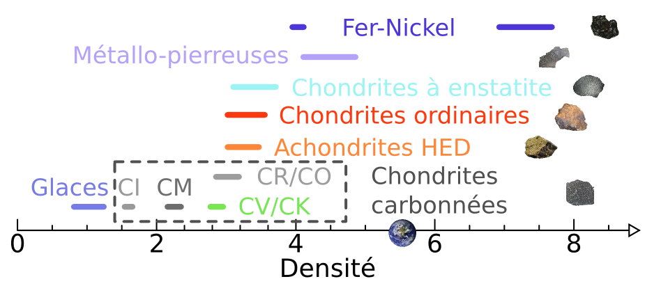
Once the mass is measured, the density can be computed. The density reflects the quantity of matter, the mass, contained within a given volume. The tricky question "What's the heaviest? A kg of leed, or a kg of feathers?" plays with that notion. In that question, the leed and the feathers of course have the same weight (1 kg), but the density of the leed being much higher than that of feathers (11300 agains 20 kg.m-3), the kilogram of feathers will occupy a much larger volume. Knowing the density of asteroids help us in constraining their composition.
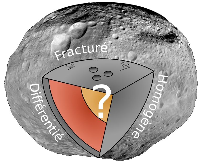
Furthermore, if the surface composition is known (see IV below), the comparison of the asteroid density with that of its constituant allows to guess its internal structure (Figure 15).
- If the asteroid is denser than its surface components, some denser compounds are located in its interior. It may indicates that the asteroid is differentiated, like (4) Vesta for instance
- If the asteroid is less dense than its surface compounds, its interior may contain less dense compounds, like ices, or large voids. Some asteroids are indeed so little dense that their density can be hardly explained without the presence of large cracs or voids in the interior.
- If the asteroid has the same density as its surface material, it is likely homogeneous.
IV. What asteroid are made of?
The study of asteroid composition is at the heart of our quest of our origins. Being the remnants of the building blocks that accreted to form the planets some 4.5 Gyrs ago, their composition tells us about the condition that reigned within the young solar system (relative abundances of elements, temperature, accretion timescales, etc).
IV.1. Means of study
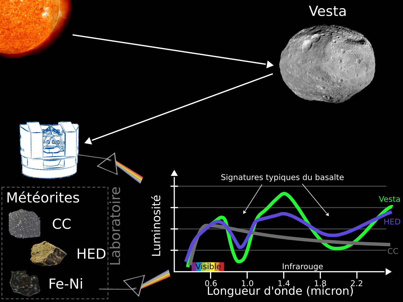
With the exception of the single sample return from the asteroids (25143) Itokawa by the Japanese mission Hayabusa in 2011, the study of asteroid composition is done remotely, by analyzing the light they reflect and by comparing it with meteorites and minerals studied in the laboratory.
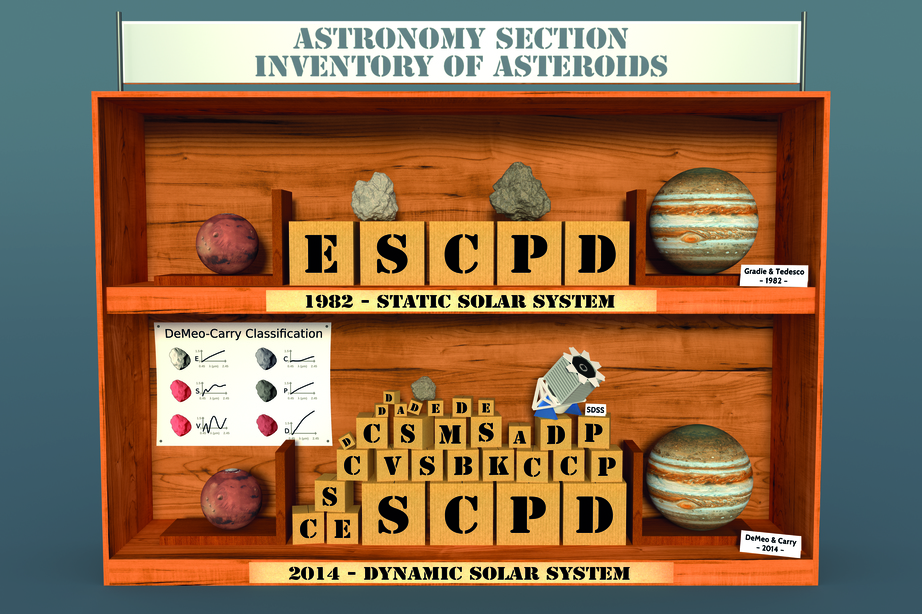
Colors of the surface: Starting in the second half of the XX century, measurements of the colors of asteroid surface revealed the existance of several groups. These measurements were conducted with broad-band filters, corresponding roughly to the red, green, and blue colors. The labels of red or blue behavior of asteroid surface is an heritage from this epoch, depending on the capability of the asteroid to reflect more light in the red of blue filter. The first classification systems, called taxonomies, of asteroids according to their surface properties were based on these colors.
Spectroscopy: By spreading the light over wavelength, one can measure its spectral distribution. It is equivalent at taking many many images, with narrow filters, each corresponding to a precise wavelength. The shape of these spectra, i.e., the distribution of the reflected light as function of the wavelength, tells us about its compounds. Matters is organized in atoms, molecules, crystals, all with well-defined frequency of quantic transition, rotation, vibration, etc. These create recognizable features in the spectra, called absorption band. Identifying these bands provide the list of surface compounds.
Albedo: Different material do not reflect the light the same way. This is fairly intuitive: this is how we define "dark" and "light" objects. The first absorbs more light than the second, which reflects more of it. This information for asteroids can also be used to identify their composition and link them with meteorites.
 
IV.2. Interpretations
The first studies of asteroid surface composition revealed that those from the inner part of the main belt (Figure 3) reflected more light and were redder than those from the outer part, bluer and darker (with a lower albedo). In the 1980s, several groups of asteroids with distinct colors, organized in distance to the sun were discovered (Gradie & Tedesco, 1982, see Figure 17). The interpretation that prevailed was that this succession was the result of a strong temperature gradient accross the belt in its early stage. But this view got more complex, with new compositionnal characteristics of the belt unveiled by more and more observations. These observations were challenging more and more this classical interpretation. A first, only a few rogue asteroids, not following the large groups succession were discovered.
Today, with over half a million of asteroids discovered since the 1980s, the availability of colors and spectra of several tens of thousands of asteroids, the idea of a static solar system has been replaced with a much more dynamical interpretation, where little things are located where they formed (see DeMeo & Carry 2014). This new interpretation was motivated by the structure of the asteroid main belt, sculpted by planetary miration. These being apparently common in exoplanet systems, our solar system most likely also witnessed changes in the orbits of planets.
Dynamical models, such as the Nice model, which try to explain the overall structure of our solar system (the orbits of the giant planets, Pluto and the transneptunian objects, and the trojan asteroids) all include a phase of planetary migration during which the giant planets have migrated over substantial distances, shaking the asteroids (which were formed everywhere in the proto-planetary disk) like snowflakes in a glass globe. The main belt is is what remain of them, from the entire solar system.
Bibliography
(Click on the link to access more bibliographic informations from the Astrophysics Data System - SAO/NASA)
- Carry et al. 2010: Physical properties of (2) Pallas, Icarus.
- Carry et al. 2012: Shape modeling technique KOALA validated by ESA Rosetta at (21) Lutetia, Planetary & Space Science.
- Carry et al. 2015: The small binary asteroid (939) Isberga, Icarus.
- Delbo et al. 2009: First VLTI-MIDI Direct Determinations of Asteroid Sizes, The Astrophysical Journal.
- DeMeo & Carry 2014: Solar System evolution from compositional mapping of the asteroid belt, Nature.
- Durech et al. 2010: DAMIT: a database of asteroid models, Astronomy & Astrophysics.
- Durech et al. 2015: Asteroid Models from Multiple Data Sources, in Asteroids IV.
- Dohnanyi 1969: Collisional Model of Asteroids and Their Debris, Journal of Geophysical Research.
- Fienga et al. 2011: The INPOP10a planetary ephemeris and its applications in fundamental physics, Celestial Mechanics and Dynamical Astronomy.
- Gradie & Tedesco 1982: Compositional structure of the asteroid belt, Science.
- Hanus et al. 2011: A study of asteroid pole-latitude distribution based on an extended set of shape models derived by the lightcurve inversion method, Astronomy & Astrophysics.
- Hanus et al. 2013: Asteroids' physical models from combined dense and sparse photometry and scaling of the YORP effect by the observed obliquity distribution, Astronomy & Astrophysics.
- Johansen & Lacerda 2010: Prograde rotation of protoplanets by accretion of pebbles in a gaseous environment, Monthly Notices of the Royal Astronomical Society.
- Kaasalainen et al. 2002: Asteroid Models from Disk-integrated Data, in Asteroids III.
- Kaasalainen 2011: Maximum compatibility estimates and shape reconstruction with boundary curves and volumes of generalized projections, Inverse Problem and Imaging.
- Lebofski et al. 1989: A refined 'standard' thermal model for asteroids based on observations of 1 Ceres and 2 Pallas, Icarus.
- Masiero et al. 2011: Main Belt Asteroids with WISE/NEOWISE. I. Preliminary Albedos and Diameters, The Astrophysical Journal.
- Morbidelli et al. 2005: Chaotic capture of Jupiter's Trojan asteroids in the early Solar System, Nature.
- Russell et al. 2012: Dawn at Vesta: Testing the Protoplanetary Paradigm, Science.
- Saint-Pé et al. 1993: Demonstration of adaptive optics for resolved imagery of solar system objects - Preliminary results on Pallas and Titan, Icarus.
- Scheeres et al. 2015: Science, in Asteroids IV.
- Thomas et al. 1997: Impact excavation on asteroid 4 Vesta: Hubble Space Telescope results, Science.
Credit : B. Carry/IMCCE/Observatoire de Paris